Biased estimators

The plan for today is to talk about an oft-neglected difference between means and standard deviations in statistics. As we will see, while means are relatively immune to over- or undershooting the true value when the sample size is low, standard deviations are a lot less robust in low-n scenarios. In this post, we will focus on seeing this property in simuated data and understanding what this could potentially mean. I will argue that, given the integral role that standard deviations play in inferential statistics,¹ we should be very aware of the detrimental effects of low-n studies.

In a later post that will be a follow-up of what we see here, we will encounter an example that illustrates the impact that the bias associated with standard deviations can have on the models we compute for our experimental data.

library(here)
library(tidyverse)
library(patchwork)
library(gghalves)

source("../../scripts/theme.R")

We will start by reviewing the two parameters that determine what a given normal distribution looks like, the mean and the standard deviation. As a second step, we will sample loads of data from distributions with known means and standard deviations and see how accurate the means and standard deviations we calculate from those sample are. When comparing means and standard deviation the often underappreciated difference in bias will emerge.

And now, onwards!

What are means and standard deviations again?

First, we will start with a plot. Imagine we ran an experiment and that the plot below shows the results for one condition from that experiment. For simplicity’s sake, we will assume that the responses we got from that imagined experiment are truly Gaussian—meaning normally distributed—, while acknowledging that these types of data are quite hard to come in linguistics. As is so often the case, the points I make below will carry over to other experiment designs and dependent variables as well, but showing what I intend to show for those data would be much more laborious to do. It is hopefully obvious that you will need to use your imagination to assign some meaning to the value of 80 you see as the mean in the plot.

Below, in addition to plotting the familiar means and confidence intervals, I also add the raw data as grey points in a narrow band and the density distribution of these data points as a blue curve. To a large extent, these two latter additions are equivalent in showing of the data that gave rise to the mean. However, for our purposes today, the curved display is much more useful and we will continue to show it in future plots (unlike the raw data points, which are only included here for readers who might be less familiar with the distributional portiom of the plot).

mean <- 80
sd <- 10
tibble(x = 1, y = rnorm(1e3, mean, sd)) %>%
    ggplot(aes(x = x, y = y)) +
    geom_half_violin(
        fill = colors[1],
        alpha = .3,
        color = NA,
        bw = 10,
        trim = FALSE
    ) +
    geom_jitter(color = "grey", size = .5, width = .01) +
    stat_summary(
        fun.data = mean_cl_normal,
        geom = "errorbar",
        width = .02,
        color = colors[1]
    ) +
    ylim(40, 120) +
    stat_summary(fun = mean, geom = "point", size = 5, color = colors[1]) +
    theme(axis.text.x = element_blank(), axis.title.x = element_blank())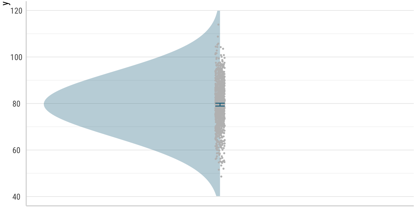

Obviously, this kind distribution is an optimistic target for a real experiment (and confidence intervals this narrow would make me and hopefully make you incredibly skeptical if this were a presented as real data). In fact, if you have a look at the code, you will see that I cheated in order to make the curve look a lot prettier than it ordinarily would be with 1000 data points. For now though, we are only interested in the shape of the curve to remind ourselves about some basic facts of distributions, so let us suspend our disbelief.

Turning the distribution around a bit and removing some of the other elements of the plot, we get this: a probability density function for data from a normal distribution with mean 80 and standard deviation 10—\(\mathcal{N}(80, 10)\). For this distribution, values very to 80 are the most likely, while values become less likely the further they lie from 80 in either direction. That is, 70 or 90 are still relatively probable but 50 and 110 are much less likely. Just have a look at the raw data points in the first plot again to confirm that this is borne out.

x1 <- mean - sd
x2 <- mean + sd
y_sd <- dnorm(x1, mean = mean, sd = sd)

ggplot() +
    stat_function(
        geom = "area",
        fun = dnorm,
        args = list(mean = mean, sd = sd),
        fill = colors[1],
        alpha = 0.3
    ) +
    geom_segment(
        aes(x = x1, xend = x2, y = y_sd, yend = y_sd),
        color = colors[2],
        linetype = "dashed"
    ) +
    annotate(
        "text",
        x = mean,
        y = dnorm(mean, mean = mean, sd = sd),
        label = paste0("μ = ", mean),
        color = colors[1],
        vjust = -0.3,
        size = 4
    ) +
    annotate(
        "text",
        x = mean,
        y = y_sd,
        label = paste0("±1 σ; σ = ", sd),
        color = colors[2],
        vjust = -.5,
        size = 4
    ) +
    theme_void() +
    xlim(40, 120)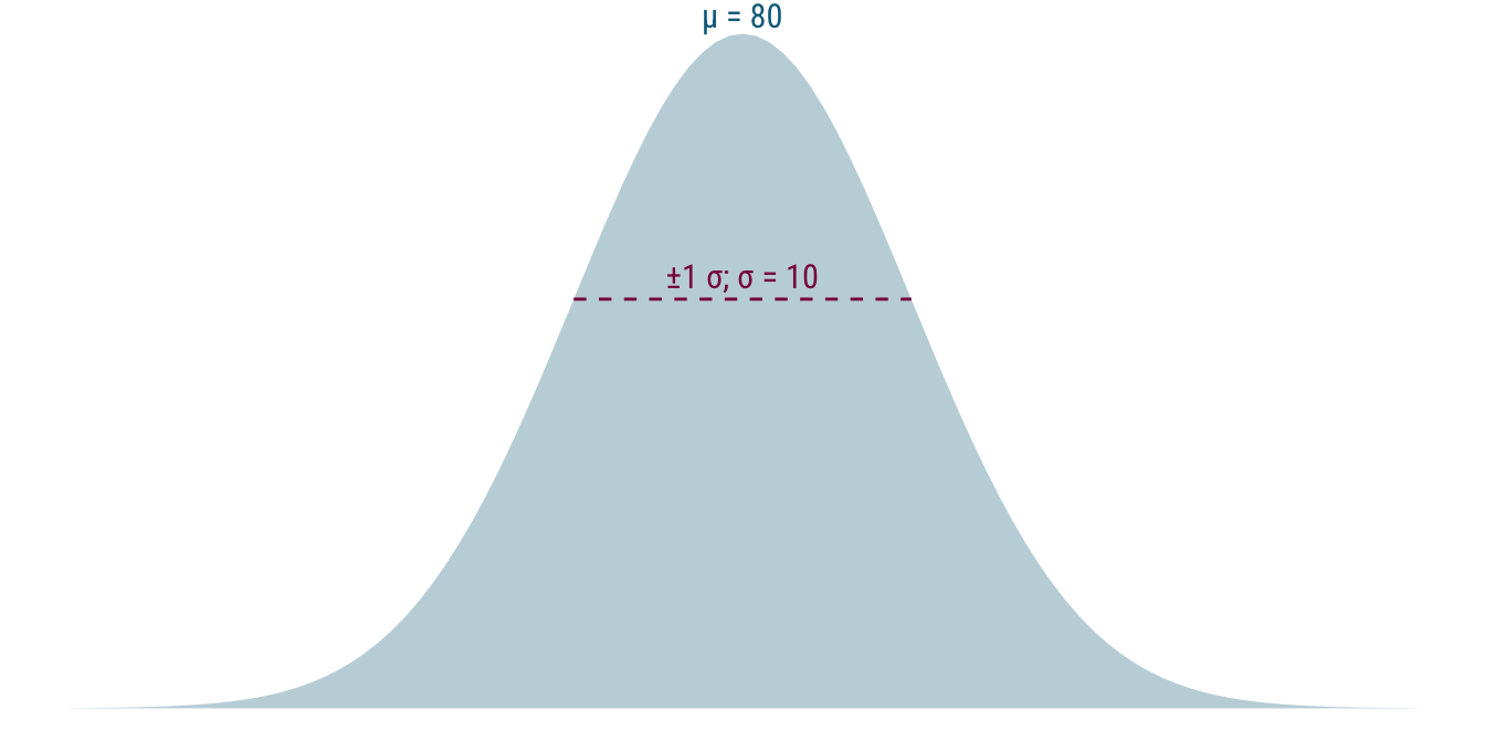

As is hopefully obvious, because we turned our distribution to the side, an increase in the mean parameter \(\mu\) will make the distribution shift further to the right. For this reason, means are also called a location parameter (of the normal distribution). The plot below illustrates this using four distinct probability distributions that only differ in terms of their location parameter \(\mu\). The scale parameter \(\sigma\), the standard deviation, is the same between all of the distributions at 10.

• \(\mathcal{N}(60, 10), \mathcal{N}(80, 10), \mathcal{N}(100, 10), \mathcal{N}(120, 10)\)

means <- c(60, 80, 100, 120)
blend_palette <- colorRampPalette(c(colors[1], colors[2]))

ggplot() +
    map2(
        means,
        blend_palette(4),
        ~ stat_function(
            geom = "area",
            fun = dnorm,
            args = list(mean = .x, sd = sd),
            fill = .y,
            alpha = 0.3
        )
    ) +
    geom_text(
        data = data.frame(
            x = means,
            y = dnorm(means, means, sd),
            label = paste0("μ = ", means)
        ),
        aes(x = x, y = y, label = label),
        vjust = -0.3,
        size = 4
    ) +
    theme_void() +
    xlim(20, 160)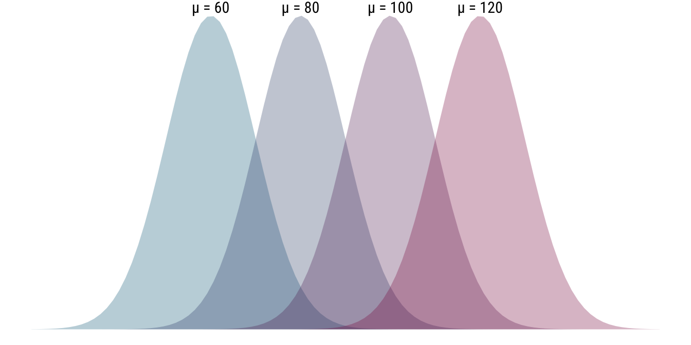

Below, we do the opposite and keep the location parameter \(\mu\) fixed at 80 while varying the scale parameter. As your can see, rather than moving the distribution to the left or right, by changing the standard deviation we are manipulating the shape of the distribution: as \(\sigma\) increases, the distribution becomes flatter and more dispersed. Conversely, a low value for \(\sigma\) indicates that the values are tightly clustered around the mean.

• \(\mathcal{N}(80, 5), \mathcal{N}(80, 10), \mathcal{N}(80, 15), \mathcal{N}(80, 20)\)

sds <- c(5, 10, 15, 20)

ggplot() +
    map2(
        sds,
        blend_palette(4),
        ~ stat_function(
            geom = "area",
            fun = dnorm,
            args = list(mean = mean, sd = .x),
            fill = .y,
            alpha = 0.3
        )
    ) +
    geom_text(
        data = data.frame(
            x = mean,
            y = dnorm(mean, mean, sds),
            label = paste0("σ = ", sds)
        ),
        aes(x = x, y = y, label = label),
        vjust = -0.3,
        size = 4
    ) +
    theme_void() +
    xlim(20, 140)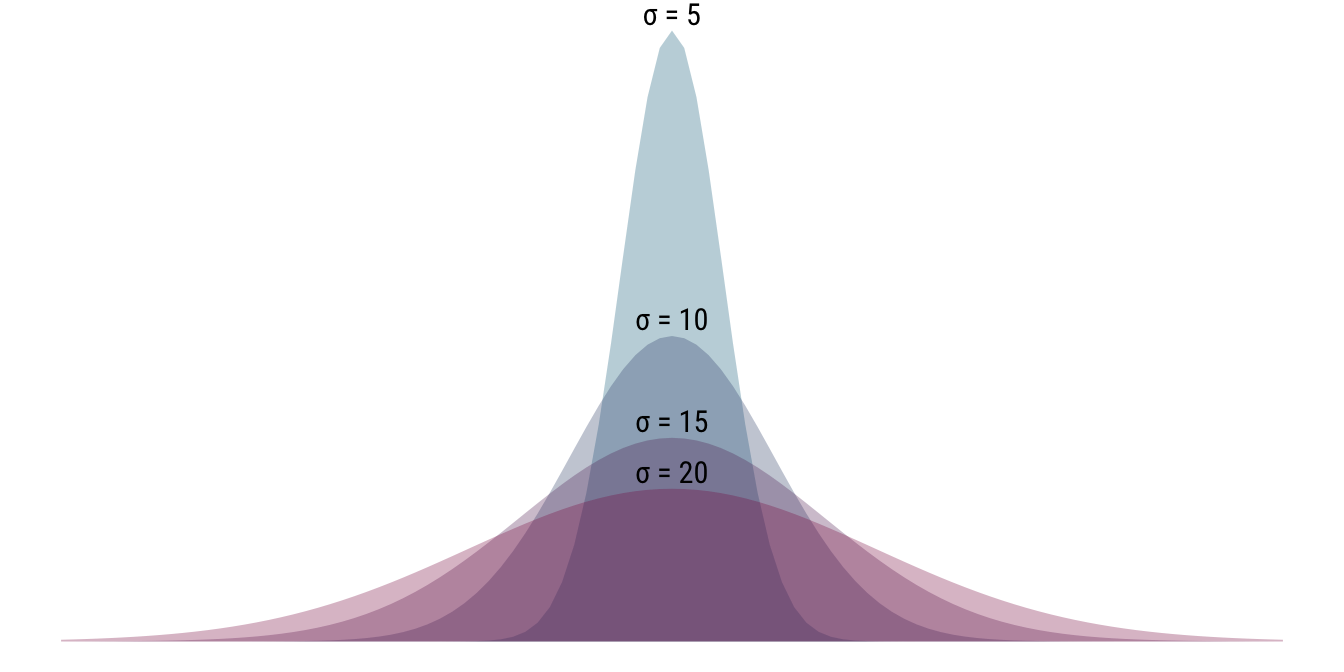

Getting to it: simulating low-n data collection runs

Now we are finally in a position to simulate some data and compute some stats. But before we head into the weeds, I briefly want to shout out my inspiration for this part of the blog post: Danielle J. Navarro’s stats book, page 318. Also go check out her fantastic blog, Notes from a data witch.

Danielle samples data from distributions with known properties, i.e., known mean and standard deviation. In our case, we will use the familiar \(\mathcal{N}(80, 10)\) that we have been looking at the entire time. This allows us to check whether the samples we obtain accurately recover, i.e., serve as good estimates of, the true parameters of the sampling distribution. So for each sample of some certain size, we calculate the mean and standard deviation. To get a sense of how it will work, here we sample 8 data points from \(\mathcal{N}(80, 10)\) and calculate our parameters of interest:

(samples <- rnorm(8, mean = mean, sd = sd))

[1] 74.514963 88.294677 78.861886 90.325240 73.201327 67.644489 82.197637 70.742368

tibble(
    mean = mean(samples),
    sd = sd(samples)
)

# A tibble: 1 × 2
   mean    sd
  <dbl> <dbl>
1  78.2  8.20

Now, since there is randomness associated with sampling from a distribution, we want to repeat this sampling and calculation process many times to ensure that our calculations are not thrown off by that randomness. In the code chunk below, we scale our operation up in two ways. First, we just sample more often: we repeat the process from above many thousands of times. Second, we vary how many data points we sample each time: above we sampled 8 data poits, below we sample from 1 to 12 data points. This is a lot of data, but we will just condense it down into one mean and standard deviation value per sample size. Here’s what we end up with:

set.seed(1234)
n_sim <- 10000
max_sample_size <- 12

sim_runs <- map(1:max_sample_size, function(n) {
    samples <- replicate(n_sim, rnorm(n, mean = mean, sd = sd))
    if (n == 1) {
        samples <- matrix(samples, nrow = 1)
    }
    sample_means <- colMeans(samples)
    sample_sds <- apply(samples, 2, sd)
    tibble(n = n, mean = mean(sample_means), sd = mean(sample_sds))
}) %>%
    list_rbind() %>%
    mutate(across(everything(), ~ replace_na(., 0)))

sim_runs

# A tibble: 12 × 3
       n  mean    sd
   <int> <dbl> <dbl>
 1     1  80.1  0   
 2     2  80.0  8.06
 3     3  80.0  8.86
 4     4  80.1  9.21
 5     5  80.0  9.30
 6     6  80.1  9.48
 7     7  80.0  9.68
 8     8  79.9  9.67
 9     9  80.0  9.74
10    10  80.0  9.74
11    11  80.0  9.76
12    12  80.0  9.75

Alright, we have our simulated data and we can sort of see what is going on. To drive home the message, let’s have ourselves a plot. Below, I define a function that makes a line plot for either the means or standard deviations we calculated from our simulated data. We will also add a horizontal dashed line that indicates the true value of the parameter in question, either 80 for the mean or 10 for the standard deviation.

The pattern that emerges is quite telling. For the means, we see that even very low sample sizes give us a pretty accurate estimate of the true mean. Of course, precision increases with sample size, but even with just a few data points, the point estimate is right on track. The standard deviations, on the other hand, show a very different pattern. As the sample size increases, the standard deviation estimates trend upwards towards the true value. For very low sample sizes, however, the standard deviation estimates are way too low. For example, when we only have two data points, the standard deviation estimate is only at about \(8\) compared to the true value of \(10\). This is the bias that I mentioned at the start of the post: the sample standard deviation is a biased estimator of the population standard deviation, particularly so for low sample sizes.

sim_plot <- function(ycol, ylab, pop_val, ylim) {
    ggplot(sim_runs, aes(x = n, y = {{ ycol }})) +
        geom_line(color = colors[1]) +
        geom_point(color = colors[1], size = 3) +
        geom_hline(
            yintercept = {{ pop_val }},
            lty = "dashed",
            color = colors[2]
        ) +
        labs(x = "Sample size", y = ylab) +
        scale_y_continuous(
            breaks = scales::breaks_pretty(),
            limits = {{ ylim }}
        ) +
        scale_x_continuous(breaks = 1:max_sample_size)
}

sim_plot(mean, "Sample mean", 80, c(79, 81)) /
    sim_plot(sd, "Sample standard deviation", 10, c(0, 10))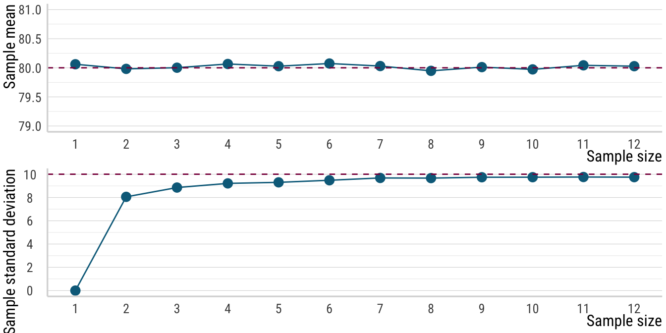

To get a clearer idea what this means, let us focus on the interpretation of standard deviations in the context of normal distributions for the moment. Below we have a curve that illustrates the percentage of values that lie within one standard deviation of the mean of the distribution. That is, the standard deviation tells us how much of the data is covered if we look at the interval from one standard deviation below the mean to one standard deviation above the mean. In a normal distribution, this interval contains about 68% of all data values.

gaussian_uder_curve <- function(sd, bound = 4) {
    # compute density across plot area values
    d <- data.frame(x = seq(-bound, bound, 0.01)) %>%
        mutate(y = dnorm(x, mean = 0, sd = 1))

    ggplot(d, aes(x = x, y = y)) +
        geom_area(
            data = filter(d, x >= max(-sd, -bound) & x <= min(sd, bound)),
            aes(x = x, y = y),
            color = colors[1],
            alpha = .3,
            fill = colors[1]
        ) +
        geom_line(linewidth = .5, color = colors[1]) +
        labs(
            subtitle = paste0(
                "Shaded area contains ",
                round(abs(pnorm(sd, 0, 1) - pnorm(-sd, 0, 1)) * 100, 1),
                "% of the data"
            )
        ) +
        theme_void() +
        theme(plot.subtitle = element_markdown(hjust = .5))
}

gaussian_uder_curve(sd = 1)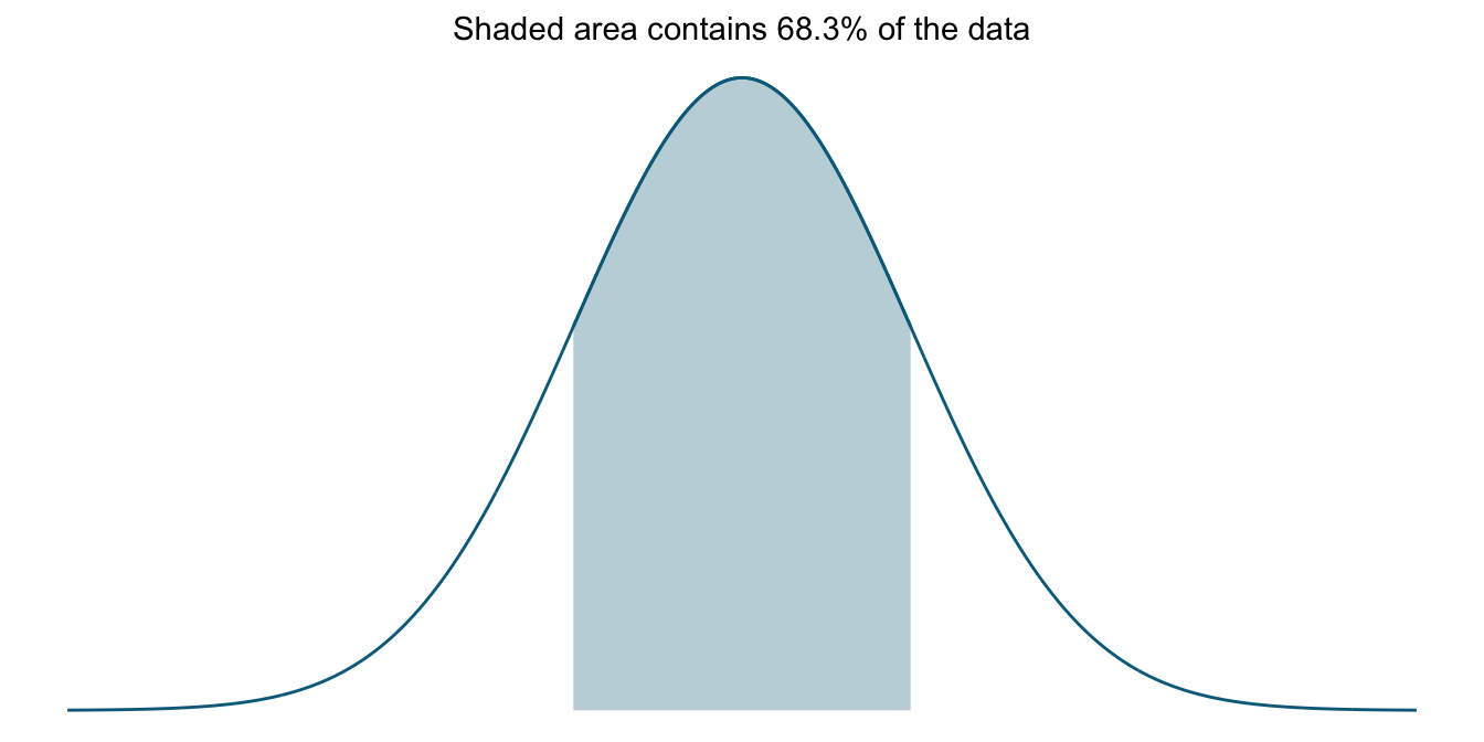

Instead, if we increase our interval to two and three standard deviations, we cover (about) 95 and 99.7 percent of data values, respectively. This is sometimes called the 68–95–99.7 rule. The two plots below show these intervals.

gaussian_uder_curve(sd = 2) /
    gaussian_uder_curve(sd = 3)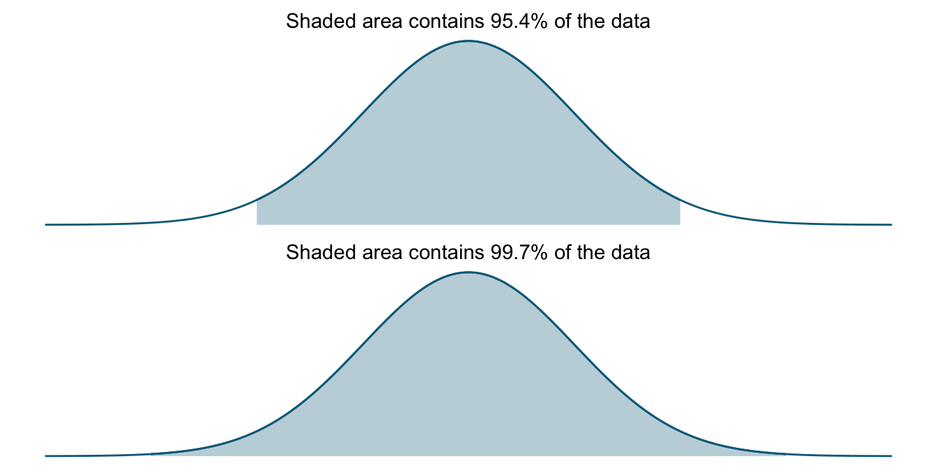

These kinds of laws are of course taken into consideration for the various statistical hypothesis tests on the market, from the \(t\)-test to more complex linear mixed models. The whole reason that the rule of thumb for \(t\) statistics exists (\(t > 2\) is significant) is that as we move two standard deviations away from the mean, we are reaching the tails of the distribution, meaning any value this far out is quite unlikely.

If we now have too few data points and systematically underestimate the standard deviation (because it is a biased estimator), our standard deviations will actually cover fewer of the values coming from the distribution than they are supposed to. Below, I illustrate this with another shaded-curve plot where I shade an interval corresponding to .8 standard deviations (with the 1 SD plot underneath to make the comparison easier). This roughly corresponds to the value we saw in our simulations for a sample size of 2 where the standard deviation was underestimated at around 80% of the true value. Here our interval covers only 57.6% of the data, in effect leaving out more than a tenth of the data it is supposed to cover.

gaussian_uder_curve(sd = .8) /
    gaussian_uder_curve(sd = 1)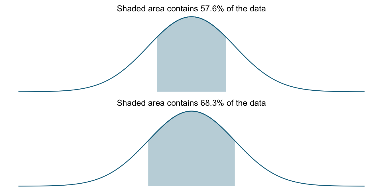

Conclusion: What does this all mean?

Since the sample standard deviation is part of the input for the computation of both standard errors of the mean and confidence intervals, the knock-on effects of an underestimated standard deviation have quite the potential for catastrophe, statistically speaking.

Consider first that every statistical test in some way puts the systematic variance in relation to the unsystematic variance. The more systematic variance, i.e., the effect of our manipulation, compared to the unsystematic variance, namely the variance that cannot be attributed to the things we controlled for, the surer we are that our manipulation had a statistically significant effect. On the flipside, if there is loads of unsystematic variance compared to the systematic variance, our tests will signal that our manipulations did not have a reliable effect.

Misestimating the standard deviation, which represents the unsystematic variance components, may thus make us draw wrong conclusions. And as we have seen, having samples that are too small is a good way of underestimating the standard deviation. This means that in low-n studies, we may be systematically underestimating the unsystematic variance and thus overestimating the systematic variance. This is a recipe for false positives, i.e., concluding that there exists a statistically significant effect where there isn’t one.

The way forward: Next time

In the next post, we will see an application of the concept of biased estimator applied to a common experiment type in linguistics. As we will see, particularly in experiments of this type, the fact that standard deviations are biased estimators will rear its ugly head and cause our inferential statistics to be so unreliable that I (and hopefully you) will wonder whether these kinds of experiments should be run in the first place.

The point will be the following: If you want to calculate \(p\)-values for data from a low-n study, it does not matter that the mean is an unbiased estimator (though of course it’s a nice thing to have). Since calculating the test statistics that the \(p\)-value will be based on involves both the mean and the standard deviation, your inferential step will be biased. So unless you use your experimental data for non-inferential processes, getting an accurate estimate for the standard deviation is necessary in order to ensure that the \(\alpha\) levels you are (or, more realistically, your field is) comfortable with—say \(\alpha = 0.05\)—actually mean what you think they mean for your experiment. Of course, if they don’t because you have too few data, your signifcant results may be nothing more than artifacts of the biased standard deviation estimator.

Lastly, for those worried that I will be shutting down their favorite experimental paradigm, don’t be. What we will have a look at is not a real paradigm, more a certain design feature that is easily changed.

References

Thalmann, Maik. in progress. Not so squeamish, Your majesty: The presuppositions of singular definites between existence and uniqueness.

Thalmann, Maik, and Andrea Matticchio. in progress. Kleene’ing up your attitude: Against universal presupposition projection.

Thalmann, Maik, and Andrea Matticchio. 2024. On being certain that presuppositions don’t project universally. In Proceedings of the Amsterdam Colloquium, 378–385.

Footnotes

1. Certainly in my own work, like Thalmann and Matticchio (2024), Thalmann and Matticchio (in progress), and Thalmann (in progress), where I explore the theoretical significance of standard deviation differences in semantics, but also in experimental linguistics and related fields more generally.