The case for precise hypotheses

We know in advance that the null hypothesis of zero effect and zero systematic error is false. This is often brought up as one of the first criticisms of the null hypothesis significance testing approach, but there is an additional error with the logic of null hypothesis significance testing. Typically, the process of hypothesis testing in this framework depends only on a precise null hypothesis, i.e., \(\theta = 0\) for some mean difference, and not on any specific alternative hypothesis, even though we generally could not care less about the null hypothesis (because we know it to be false). We accept an alternative hypothesis simply when \(\theta \neq 0\). But since in practice we know that the null hypothesis is false from the get go, rejecting that competitor is trivial and uninformative: every effect is different from zero, at least to some minuscule degree. Thus, rejecting the null is simply a question of sample size: at some point, your p-value will clear your \(\alpha\) threshold. Accepting a non-null hypothesis is thus just a matter of time and money under this approach.

But this is not just an issue with p-values, it is also an issue with how we view hypotheses in general. If we allow ourselves to consider imprecise alternative hypotheses—namely one that we consider accepted already when \(\theta \neq 0\).—, we may miss theoretical issues with the hypothesis we consider a potential model of the world that we could have anticipated even before designing the experiment. An imprecise theory will often be flexible enough to accommodate just about any data we might collect, and thus will not be informative. In other words, if it doesn’t matter from the perspective of our ‘theory’ whether \(\theta > 0\) or \(\theta < 0\), then maybe we should give that model a second look. In turn, the experiment will not be informative either, because the theory is ill-defined for testing to begin with. This is a point that Meehl (1967) made forcefully in his critique of psychological theories (which he contrasts with theories in physics): the should ultimately be the falsification of one’s pet theory (and then further refinement), rather than mere confirmation by defeating a straw man.

In today’s short post, I want to raise awareness for certain issues that are connected with the way we typically view and use hypotheses in frequentist paradigms (though this will not be a critique of frequentism; we could easily reproduce these issues in a Bayesian fashion):

1. If possible, we should contrast real competitor theories rather than alterative and null hypotheses.
2. Imprecise hypotheses may be theoretically malformed.
3. Plotting the set of hypotheses to be tested, compared to giving expectations of effects in math talk, makes it easier to spot the previous issue and makes a publication more understandable to non-expert or non-statistician readers.
4. As experiments grow in complexity—say beyond the classical \(2 \times 2\)—, it becomes increasingly difficult to interpret predictions that are only given as coefficients.

library(here)
library(patchwork)
library(tidyverse)
library(gghalves)
library(broom)

source("../../scripts/theme.R")

Towards precision and real competition

What’s the alternative? We need to compare theories that make precise predictions against each other. That is, each theory should be a real contender, not just some statistical straw man that we can shadowbox against. In this way, we subject each model to a severe test—one that has a realistic chance to fail—where its falsification is informative for our field of study, rather than being a foregone conclusion. For an idea that goes in this direction, see Dongen et al. (2023).

However, even in the absense of two competing hypotheses, which simply may not be available in all cases, there are advantages to being concrete about experimental predictions rather than relying on the built-in precision of the null hypothesis inherent to significance testing. As I said before, it works as a safeguard: by completely specifying where every condition mean is predicted to land when the data are collected and why, you get a sense of the completeness of the theory or at least your interpretation of it. This, in turn, allows you to assess its a priori sensibility.

But arguably the more important advantage is that precision facilitates communication to audiences that might not be quite as familiar with the subject matter but still have a vested interest in the outcome of your study. Or, probably more relevantly in linguistics, it allows readers who are not familiar with experimental and statistical techniques to quickly assess whether your data are in support or in violation of the theoretical predictions outside of statistical summary values. While an experimentalist is likely able to translate the foregoing theoretical discussion and the experimental design into a prediction about statistical effects, a theoretician may not have as easy of a time with this.

But when you say that the theoretical account you’re attempting to falsify predicts an interaction between factors \(W\) and \(Z\) of \(\theta > .5\), even readers with only passing knowledge of statistics may be able to check your model summaries for the \(W:Z\) effect in question and evaluate whether your results cleared that bar (with sufficient distance not to be of a spurious nature). In absence of this statement of the theoretical prediction in statistical terms, a reader may inadvertently miss that a significant effect for \(W:Z\) is not in support but in conflict with the state of affairs the theory allows for. Or they may take a data point that a theory is silent on as being in support simply because that effect is statistically significant—even though this only means that it likely conflicts with the null hypothesis.

The case for hypothesis plots

Even better, if you plot the patterns that the theory predicts in the same style as your summary figure for the experimental results, readers will easily be able to check what the results means in terms of the predictions, potentially without having to interpret any statistical summary values. This way any reader will be able to immediately check whether, in their view, the (or any) hypothesis fits the data.

In the ideal case, a hypothesis plot should make it possible to evaluate the question whether the experimental data are in support or in conflict with a theoretical position at a glance, to some extent even without domain knowledge. To see what I mean, consider the plot below, which details the legitimate predictions of two competing hypotheses in formal semantics for the question of how presuppositions project from quantified environments (see Thalmann and Matticchio submitted; Thalmann and Matticchio 2024 for a proper description of what is going on with these theories and the experiment).

preds <- tribble(
    ~"Scenario", ~"Negation", ~"Judgment", ~"who",
    "true", "without", 2, "*again*<br>Strong Kleene",
    "true", "without", 2, "*again*<br>Universal Projection",
    "true", "with", -2, "*again*<br>Strong Kleene",
    "true", "with", -2, "*again*<br>Universal Projection",
    "false", "without", -2, "*again*<br>Strong Kleene",
    "false", "without", -2, "*again*<br>Universal Projection",
    "false", "with", 2, "*again*<br>Strong Kleene",
    "false", "with", 2, "*again*<br>Universal Projection",
    "undef.", "without", 0, "*again*<br>Strong Kleene",
    "undef.", "without", 0, "*again*<br>Universal Projection",
    "undef.", "with", 0, "*again*<br>Strong Kleene",
    "undef.", "with", 0, "*again*<br>Universal Projection",
    "crit.", "without", -2, "*again*<br>Strong Kleene",
    "crit.", "with", 2, "*again*<br>Strong Kleene",
    "crit.", "without", 0, "*again*<br>Universal Projection",
    "crit.", "with", 0, "*again*<br>Universal Projection",
)

p_hyp <- preds %>%
    mutate(Negation = fct_relevel(Negation, "without")) %>%
    ggplot(aes(
        x = fct_inorder(Scenario),
        y = Judgment,
        color = Negation,
        shape = Negation,
        group = Negation
    )) +
    geom_line() +
    geom_point(size = 3) +
    scale_y_continuous(
        breaks = c(-2, 0, 2),
        labels = c("Compl. false", "Neither nor", "Compl. true")
    ) +
    labs(
        x = "Scenario",
        y = "Judgment"
    ) +
    coord_cartesian(clip = "off") +
    facet_wrap(~who) +
    theme(
        legend.position = "bottom",
        axis.text.y = element_markdown(hjust = 1),
        legend.margin = margin(-25, 0, 0, 0, "pt"),
        axis.text.x = element_markdown(family = "Cascadia Code"),
        strip.text.x = element_markdown(family = "Minion Pro")
    )
p_hyp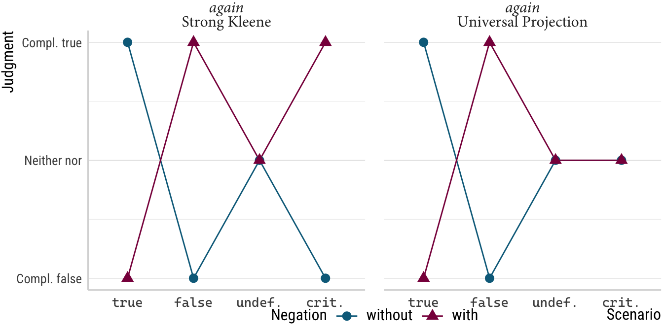

Importantly, both theoretical accounts make predictions for all eight conditions in the design, that is, for all four levels of the scenario factor in the negated and unnegated version of the critical stimulus. This allows for plenty of chances for falsification of either theory: if the actual results for the true, false or undefined scenarios depart from the predicted ones here, we have good reasons to reject either theory, as these represent non-negotiable control conditions. Only if the those six conditions turn out the way they should can we turn to theory comparison and look at what happens with the means for the critical scenarios under both settings of the negation factor. If critical and false pattern together, the Strong Kleene hypothesis has the edge and if critical looks more like the undefined scenario, the data support the Universal Projection hypothesis. That is, if we were to reduce the experiment to only include the scenarios critical and undefined as well as negation, Strong Kleene predicts an interaction. Universal Projection, on the other hand, predicts that this interaction term should be zero. Any other pattern—say one where critical patterns with true—and both theories are falsified and make wrong predictions for the actual linguistic behavior of the kinds of speakers included in the experiment.

Notice how much I had to write to communicate even a small sense of the requirements that these hypotheses place upon the data. In the hypothesis plot above, all of this work (and more, by relating it the actual scale used in the experiment) is done visually in the plot below. Detailing this in terms of effects from a model would be even more cumbersome than writing it out since this is all relative to the likelihood assumed by the model and the contrast coding of the scenario factor. Even deciding which main effects and interactions to select for such a presentation is no small feat, and that’s just the first step!¹

Now, compare the plot of the experimental results below to the plot above. Notice first that the layout is roughly the same, the only difference being that distributional and variance-related elements occur only in the plot for the actual data but are absent in the hypothesis plot where predictions for these components are absent. I would argue that it requires very little domain knowledge in formal semantics to evaluate which of two hypothesis aligns more closely with the empirical picture the experiment found. I am not denying that more thigns are relevant to the interpretation of these data, of course. To more fully appreciate the experimental results, some training in linguistics is required and to arrive at a final interpretation, maybe some stats knowledge is necessary too. My only point is that communicating these complexities is far easier against the background of precise and plotted predictions.

d <- read_csv(
    here("data", "believe-projection.csv"),
    show_col_types = FALSE
) %>%
    filter(sub_exp == 1) %>%
    mutate(
        judgment = judgment - 50,
        judgment = judgment / 25,
        scenario = gsub("undef", "undefined", scenario),
        scenario = fct_relevel(
            scenario,
            "true",
            "false",
            "undefined",
            "critical"
        ),
        negation = fct_relevel(negation, "pos"),
        negation = fct_recode(negation, without = "pos", with = "neg"),
        trigger = paste0("*", trigger, "*"),
        trigger = fct_relevel(trigger, "*again*", "*stop*"),
    )
p <- d %>%
    ggplot(aes(
        x = scenario,
        y = judgment,
        color = negation,
        fill = negation,
        pch = negation,
        group = negation
    )) +
    geom_half_violin(
        data = . %>% filter(negation == "without"),
        mapping = aes(group = scenario),
        adjust = .7,
        alpha = .2,
        fill = colors[1],
        bw = .4,
        color = "transparent",
        trim = FALSE,
        scale = "count"
    ) +
    geom_half_violin(
        data = . %>% filter(negation == "with"),
        mapping = aes(group = scenario),
        adjust = .7,
        alpha = .2,
        fill = colors[2],
        bw = .4,
        color = "transparent",
        trim = FALSE,
        scale = "count",
        side = "R"
    ) +
    stat_summary(fun = mean, geom = "line") +
    stat_summary(
        fun.data = mean_cl_normal,
        width = .15,
        alpha = .7,
        geom = "errorbar"
    ) +
    stat_summary(fun = mean, geom = "point", size = 4) +
    labs(
        x = "Scenario",
        y = "Judgment \u00B1CI<sub>95</sub>",
        color = "Negation",
        fill = "Negation",
        group = "Negation",
        pch = "Negation"
    ) +
    scale_y_continuous(limits = c(-2, 2)) +
    theme(
        legend.margin = margin(-25, 0, 0, 0, "pt"),
        axis.text.x = element_markdown(family = "Cascadia Code")
    )
p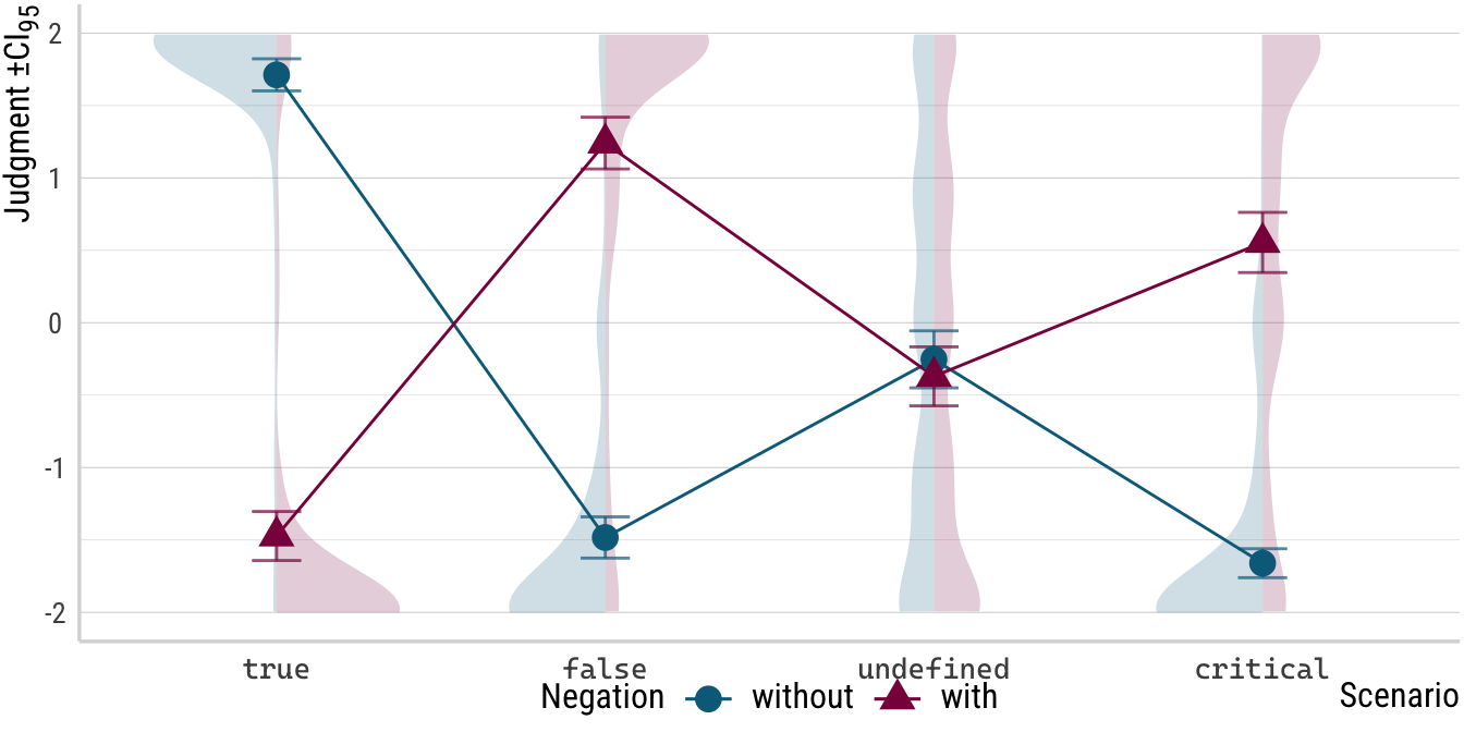

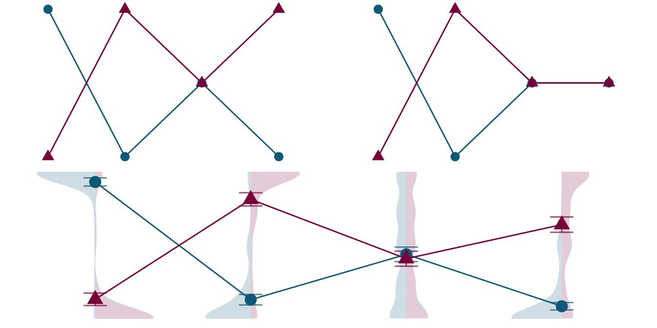
Just for fun, below we have a combined figure without the otherwise helpful labels. In my mind, the point from above still stands: if you know that you’re supposed to decide which hypothesis from the top panel is right based only on these plots, the job does not seem to be too taxing and the left plot from the top row seems like the obvious choice. Of course, removing the label does not yield a great approximation of how a person must feel who’s not so confident reading your paper, but it is my hope that it goes in the right direction.

wrap_plots(
    p_hyp +
        theme_void() +
        theme(strip.text.x = element_blank()) +
        guides(color = "none", shape = "none"),
    p +
        theme_void() +
        guides(color = "none", shape = "none", fill = "none"),
    ncol = 1
)

Confusing coefficient tables and plots

Before I stop the badgery, if you still don’t believe me that a plot is easier than mentioning coefficients, I offer a little self-experiment. Below we have a table that would adequately report the expected effects of the two hypotheses we saw above as predicted model coefficients. To do this, I encoded the expected condition means as integers in the datasets hyp_un and hyp_sk. On the assumption of a linear model with simple treatment coding, I then simply fed these data into lm() and arranged the coefficients side-by-side.

hyp_un <- tribble(
    ~"scenario", ~"negation", ~"judgment",
    "true", "without", 2,
    "true", "with", -2,
    "false", "without", -2,
    "false", "with", 2,
    "undefined", "without", 0,
    "undefined", "with", 0,
    "critical", "without", 0,
    "critical", "with", 0
)

hyp_sk <- tribble(
    ~"scenario", ~"negation", ~"judgment",
    "true", "without", 2,
    "true", "with", -2,
    "false", "without", -2,
    "false", "with", 2,
    "undefined", "without", 0,
    "undefined", "with", 0,
    "critical", "without", -2,
    "critical", "with", 2
)

coefs_treat <- lm(judgment ~ scenario * negation, data = hyp_un) %>%
    tidy() %>%
    mutate(estimate = round(estimate, 1)) %>%
    select(term, `Universal Projection` = estimate) %>%
    left_join(
        lm(judgment ~ scenario * negation, data = hyp_sk) %>%
            tidy() %>%
            mutate(estimate = round(estimate, 1)) %>%
            select(term, `Strong Kleene` = estimate),
        by = "term"
    )
coefs_treat

# A tibble: 8 × 3
  term                              `Universal Projection` `Strong Kleene`
  <chr>                                              <dbl>           <dbl>
1 (Intercept)                                            0               2
2 scenariofalse                                          2               0
3 scenariotrue                                          -2              -4
4 scenarioundefined                                      0              -2
5 negationwithout                                        0              -4
6 scenariofalse:negationwithout                         -4               0
7 scenariotrue:negationwithout                           4               8
8 scenarioundefined:negationwithout                      0               4

If I were asked to check, on the basis of these coefficient displays alone, whether the theories in question make sensible predictions according to how I take linguistic semantics to work, I would certainly be busy thinking for a while. Not so with the plotted predictions where I would expect semanticists to be quite confident and quick about their assessment.

Unsuprisingly, this issue persists (and even worsens) when we change the contrast coding to sum contrasts:

coefs_sum <- lm(
    judgment ~ scenario * negation,
    data = hyp_un,
    contrasts = list(
        scenario = contr.sum,
        negation = contr.sum
    )
) %>%
    tidy() %>%
    mutate(estimate = round(estimate, 1)) %>%
    select(term, `Universal Projection` = estimate) %>%
    left_join(
        lm(
            judgment ~ scenario * negation,
            data = hyp_sk,
            contrasts = list(
                scenario = contr.sum,
                negation = contr.sum
            )
        ) %>%
            tidy() %>%
            mutate(estimate = round(estimate, 1)) %>%
            select(term, `Strong Kleene` = estimate),
        by = "term"
    )
coefs_sum

# A tibble: 8 × 3
  term                `Universal Projection` `Strong Kleene`
  <chr>                                <dbl>           <dbl>
1 (Intercept)                              0             0  
2 scenario1                                0             0  
3 scenario2                                0             0  
4 scenario3                                0             0  
5 negation1                                0             0.5
6 scenario1:negation1                      0             1.5
7 scenario2:negation1                      2             1.5
8 scenario3:negation1                     -2            -2.5

Before concluding, I just want to add that the difficulty we detect with coefficients has very little to do with the fact that they were presented in a tabular format. Below, both sets of coefficients are plotted and I would argue that this change in presentation does not put it on equal footing with the hypothesis plot from above.

coef_plot <- function(coefs, title) {
    coefs %>%
        pivot_longer(
            cols = c(`Universal Projection`, `Strong Kleene`),
            names_to = "Hypothesis",
            values_to = "Coefficient"
        ) %>%
        ggplot(aes(
            y = fct_rev(term),
            x = Coefficient,
            color = Hypothesis,
            shape = Hypothesis
        )) +
        geom_vline(xintercept = 0, lty = "dashed", color = "grey") +
        geom_point(size = 3) +
        labs(y = "Parameter", title = title) +
        theme(
            axis.text.y = element_markdown(family = "Cascadia Code", hjust = 0)
        )
}
coef_plot(coefs_treat, "Treatment-coded coefficient predictions") /
    coef_plot(coefs_sum, "Sum-coded coefficient predictions") +
    plot_layout(guides = "collect")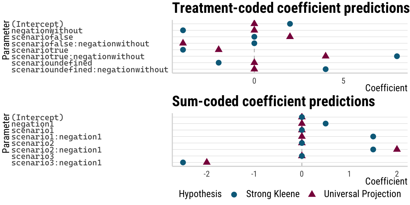

(I realize of course that this plot would be easier to interpret if the \(y\)-axis labels were changed. I was just to lazy to do it here without any real benefit: even the best labels will not make these plots easier to parse than the plotted condition mean predictions above.)

Conclusions

The call to action for this post then is to ask everybody for hypothesis plots. While I do think that null hypothesis significance testing should continue to be critically regarded as a research practice, I understand that switching the way one does stats is not easy. In the same vein, sometimes there simply aren’t multiple realistic contender hypotheses. However, if we do an experiment and we intend to run stats on the data from that experiment, it should be possible to show the expected pattern (for the one hypothesis we do have) graphically.

As we discussed, this should have two primary benefits, one for the creator and one for the eventual consumer of the paper. The creator of the plot (and the designer of the experiment) has an immediate tool for (and record of) theory interpretation and operationalization. This record also safeguards against forgetting how one interpreted the theory a few months ago, or (inadvertently) changing ones views to align with the experiment results once they’re finally collected. The consumer instead is aided with an easy-to-understand figure she can compare to the descriptive results of the experiment, no stats knowledge needed. And hopefully a paper that is understood better has a better chance of being taken into account (and cited) in the future.

References

Dongen, Noah van, Jan Sprenger, and Eric-Jan Wagenmakers. 2023. A Bayesian perspective on severity: Risky predictions and specific hypotheses. Psychonomic Bulletin & Review 30. Springer Science; Business Media LLC: 516–533. https://doi.org/10.3758/s13423-022-02069-1.

Meehl, Paul E. 1967. Theory-testing in psychology and physics: A methodological paradox. Philosophy of science 34. Cambridge University Press: 103–115.

Thalmann, Maik, and Andrea Matticchio. submitted. Kleene’ing up your attitude: Against universal presupposition projection.

Thalmann, Maik, and Andrea Matticchio. 2024. On being certain that presuppositions don’t project universally. In Proceedings of the Amsterdam Colloquium, 378–385.

Footnotes

1. Stay tuned till the end to see what a complete coefficient prediction set would look like and judge for yourself whether you’d be happy to have to puzzle out what it means as the reader of a paper.