The likelihood principle, stopping rules, and \(p\)-values

library(here)
library(patchwork)
library(tidyverse)

source("../../scripts/theme.R")

In this post, I will merely be rehashing, to the best of my ability, the well-known issue of the likelihood principle and the question of what \(p\)-values have to do with it.

While the post includes a bit of math, the main point is to illustrate the tension between \(p\)-values and the likelihood principle, and to show how this tension follows from what \(p\)-values represent. My hope is that the simulated data and the visualizations make the issue apparent and relatively intuitive, even without the math.

For some background reading, I recommend: Wagenmakers (2007) and Wagenmakers et al. (2019).

Background

Likelihood principle

The likelihood principle states:

1. Likelihood principle
   All the information in the data relevant to inference about a parameter is contained in the likelihood function.

Because of this, if two experiments yield proportional likelihood functions for the parameter of interest, they must lead to the same inferential conclusions. Formally, if two experiments \(E_A\) and \(E_B\) with observed data \(x_1\) and \(x_2\) satisfy

\[ L(\theta \mid x_1, E_A) \propto L(\theta \mid x_2, E_B) \]

for all parameters \(\theta\), then any valid inference about \(\theta\) should be identical under the two experiments. Put another way, the likelihood principle asserts that the method of data collection (e.g., stopping rules, see below) should not affect the inference drawn from the data, as long as the likelihood functions are proportional: any hypothesis test, confidence interval, or Bayesian posterior derived from \(E_A\) should be the same as that derived from \(E_B\) if the likelihood principle is satisfied.

That is, the likelihood can be defined as \(L(\theta \mid \text{observed data})\), a function of \(\theta\) with the data fixed.

Stopping rules

For anybody who started their statistics education with frequentist methods, the suggestion that the method of data collection should not affect inference is likely to be surprising, if not outright counterintuitive. After all, we are often taught that various things that have nothing to do with the observed data affect the validity of our inferences. Stopping rules are a prime example of this. A stopping rule is a pre-specified rule that determines when data collection ends. It specifies the condition under which sampling stops, based on the information observed so far.

Possible stopping rules are:

1. We will stop collecting data once we tested \(N = 50\) participants.
2. We will stop collecting data once the estimate for our parameter of interest \(\theta\) reaches a certain threshold.

The case I want to make here is that in systems that respect the likelihood principle, stopping rules and other procedural details of data collection should not affect the inference drawn from the data (as long as the likelihood functions are proportional). In these systems, stopping rules are irrelevant once the data are observed because unobserved outcomes do not matter for inference. Because of this, only the likelihood is inferentially meaningful.

Bayesian inference and likelihood-ratio methods satisfy the likelihood principle. Classical frequentist methods, which rely on \(p\)-values for inferences, generally do not because the sampling distribution for our experiment matters, and stopping rules change the sampling distribution.

The sampling distribution

While it sounds complicated, the sampling distribution is just the distribution of a statistic (e.g., a test statistic) under repeated sampling from the population.

2. Sampling distribution
   A sampling distribution is the probability distribution of a statistic \(\theta\) computed from all possible samples drawn from a population under a specified sampling process.

If our stopping rule says that we only stop collecting data once we reach \(\theta > c\) for some threshold \(c\), there will trivially be no \(\theta < c\). This changes the potential outcomes of the experiment—because we will never observe \(\theta < c\) under that stopping rule—and thus the sampling distribution, which will be truncated below \(c\). Instead, if our stopping rule gives us only a fixed sample size \(N\) (as is more common), it is certainly possible to get a \(\theta < c\).

Simply put, our stopping rules may affect the sampling distribution of the test statistic \(\theta\) in our experiment. Recall, though, that the stopping rule is independent of the likelihood, which only takes into account the observed data, not the sampling rules we adhered to when collecting those data. To restate this against the expanded background, the likelihood principle asserts that inference should depend only on the likelihood (i.e., the observed data), whereas frequentist \(p\)-values are defined using sampling distributions (i.e., the full data-generating process, which in our case includes the stopping rule), thus violating the likelihood principle.

An example with normally distributed data

With this more technical backdrop in place, we can now illustrate the difference between likelihood-based inference and \(p\)-value-based inference in the context of two experiments with normally distributed data, one with a fixed sample size and one with an optional stopping rule. We will see that the likelihoods are comparable, being unaffected by the stopping rule, but the \(p\)-values differ because of the effect that stopping rules have on the sampling distribution.

Our data will be defined as follows, with known \(\sigma^2\). As is standard, the parameter of interest, our \(\theta\), is the mean \(\mu\) of that normal distribution.

\[ X_1, X_2, \dots \sim \mathcal{N}(\mu, \sigma^2) \]

In the first example, our stopping rule will simply specify a sample size \(n\) at which data collection stops. Suppose that the sample mean satisfies \(\bar{X}_n = c\).

The likelihood is a Gaussian one, centered at \(c\), the sample mean.

\[ L_A(\mu) \propto \exp\left(-\frac{n}{2\sigma^2}(c-\mu)^2\right) \]

I will not go into this formula in detail here, but it can be derived from the one below, which might be more familiar. This likelihood is built from squared deviations \((X_i-\mu)^2\), which aggregate into a total sum of squares \(\sum_{i=1}^n (X_i-\mu)^2\), scaled by the variance \(\sigma^2\). The factor \(1/\sqrt{2\pi\sigma^2}\) is the normalizing constant that makes each term a valid normal density, which we often ignore in least squares computations.

\[ L(\mu) = \prod_{i=1}^{n} \frac{1}{\sqrt{2\pi\sigma^2}} \exp\!\left(-\frac{(X_i-\mu)^2}{2\sigma^2}\right) \]

In our second example, we will have a stopping rule that characterizes a threshold for \(c\), meaning we keep sampling until the sample mean first reaches or exceeds \(c\):

\[ N = n \text{ if and only if } \bar{X_n} ​\ge c \text{ and } \bar{X_k}​ < c \text{ for all } k=1,\dots,n−1 \]

Obviously, given that stopping rule, at the stopping time, \(\bar{X}_N = c\). For this experiment, the likelihood for \(\mu\) given this observed value is (again)

\[ L_B(\mu) \propto \exp\left(-\frac{N}{2\sigma^2}(c-\mu)^2\right). \]

Comparing the two likelihood functions, \(L_A(\mu)\) and \(L_B(\mu)\), we see that the two likelihoods are proportional:

\[ L_A(\mu) \propto L_B(\mu) \]

In principle, this should not be surprising, because the likelihood only depends on the observed data (the sample mean at stopping), and not on the stopping rule or the sampling distribution: there is no place in the formula where a stopping rule could feature. If we only look at the observed data and have no information about how the data were collected, we cannot distinguish between the two experiments. This is precisely what the likelihood principle is supposed to capture: the idea that inference should depend only on the observed data, not on the method of data collection.

Because the likelihoods are proportional, the maximum likelihood estimator of \(\mu\) is \(c\) in both cases. And because they are proportional, the likelihood ratio for any two values of \(\mu\) is the same in both experiments. Moreover, if we were to use a Bayesian approach with the same prior distribution for \(\mu\), we would get the same posterior distribution in both cases. Only an inference method that depends on the sampling distribution, such as \(p\)-values, would yield different results between the two experiments.

Thus, according to the likelihood principle, the two experiments provide the same evidence about our parameter of interest \(\mu\) (i.e., \(\theta\)).

Below, we will simulate data from both experiments to illustrate the difference between the likelihoods and the \(p\)-values. For the first few rows of the data sets below, compare especially the difference in the sample size (which is fixed at \(n\) in the first experiment and random in the second).¹

set.seed(1234)

mu0 <- 0
sigma <- 1
n <- 50
c <- 0.3 # observed sample mean / decision boundary
nsim <- 10000
max_n <- 5000

fixed_df <- tibble(
    sim = 1:nsim,
    xbar = map_dbl(sim, ~ mean(rnorm(n, mu0, sigma)))
)

optional_stop <- function(c, mu, sigma, max_n) {
    s <- 0
    for (i in 1:max_n) {
        s <- s + rnorm(1, mu, sigma)
        if (s / i >= c) {
            return(tibble(N = i, xbar = s / i))
        }
    }
    tibble(N = max_n, xbar = s / max_n)
}
stop_df <- map_dfr(
    1:nsim,
    ~ optional_stop(c, mu0, sigma, max_n),
    .id = "sim"
) %>%
    mutate(sim = as.integer(sim))
fixed_df %>%
    mutate(n = n, .after = sim)

# A tibble: 10,000 × 3
     sim     n     xbar
   <int> <dbl>    <dbl>
 1     1    50 -0.453  
 2     2    50  0.140  
 3     3    50  0.0200 
 4     4    50  0.0625 
 5     5    50  0.211  
 6     6    50  0.0986 
 7     7    50  0.00694
 8     8    50 -0.0231 
 9     9    50 -0.116  
10    10    50  0.0727 
# ℹ 9,990 more rows

stop_df

# A tibble: 10,000 × 3
     sim     N     xbar
   <int> <dbl>    <dbl>
 1     1  5000 -0.0115 
 2     2     1  0.760  
 3     3     2  0.792  
 4     4  5000 -0.0147 
 5     5  5000 -0.00942
 6     6     1  0.909  
 7     7     1  0.748  
 8     8     4  0.496  
 9     9     1  0.326  
10    10  5000  0.0129 
# ℹ 9,990 more rows

And here are the sampling distributions of the sample mean under the two experiments. Note that the distribution of the sample mean under the fixed-\(n\) design is Gaussian (as indicated by the curve), while the distribution of the sample mean at stopping under the optional-stopping design is not Gaussian, being truncated below \(c\) and having a heavier tail above \(c\).

p_1 <- fixed_df %>%
    ggplot(aes(x = xbar)) +
    stat_function(
        fun = dnorm,
        color = colors[1],
        args = list(mean = mu0, sd = sigma / sqrt(n)),
        linewidth = 1
    ) +
    geom_histogram(
        aes(y = after_stat(density)),
        bins = 50,
        fill = alpha(colors[1], .3),
        color = "white"
    ) +
    labs(
        title = "Fixed-sample Gaussian experiment",
        subtitle = "Under H<sub>0</sub>, the sample mean has an exact normal distribution.<br>This null distribution ignores how the observed value was reached",
        x = "Sample mean",
        y = "Density"
    )
p_2 <- stop_df %>%
    ggplot(aes(x = xbar)) +
    geom_histogram(
        aes(y = after_stat(density)),
        bins = 50,
        fill = alpha(colors[1], .3),
        color = "white"
    ) +
    geom_vline(xintercept = c, linewidth = 1, color = colors[2]) +
    labs(
        title = "Optional-stopping Gaussian experiment",
        subtitle = "Under H<sub>0</sub>, the distribution of the stopping-time mean is non-normal.<br>It reflects boundary crossing (indicated by red line), not fixed-sample averaging",
        x = "Sample mean at stopping",
        y = "Density"
    )
p_1 / p_2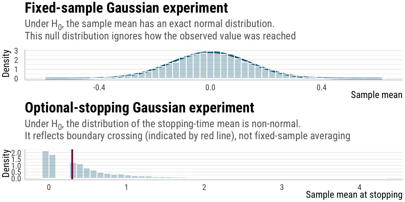

But not just the distributions above differ, the sample size also differs between the two experiments. In the fixed-\(n\) design, the sample size is always \(n\), while in the optional-stopping design, the sample size \(N\) is random and typically smaller than \(n\), except for when the sample mean does not reach \(c\) within the maximum number of samples, in which case \(N\) is equal to the maximum number of samples. This is shown below.

p_3 <- ggplot(stop_df, aes(x = N)) +
    geom_histogram(bins = 50, fill = alpha(colors[1], .3), color = "white") +
    scale_x_continuous(
         trans = scales::pseudo_log_trans(base = 10),
         breaks = c(1, 10, 100, 1000, 5000)
     ) +
    labs(
        title = "Distribution of the stopping time under H<sub>0</sub>",
        subtitle = "The stopping time has a heavy-tailed distribution which invalidates normal approximations.<br>The peak at *N* = 5000 is due to the maximum sample size",
        x = "Stopping time (N), pseudo-log scale",
        y = "Number of simulations"
    )
p_3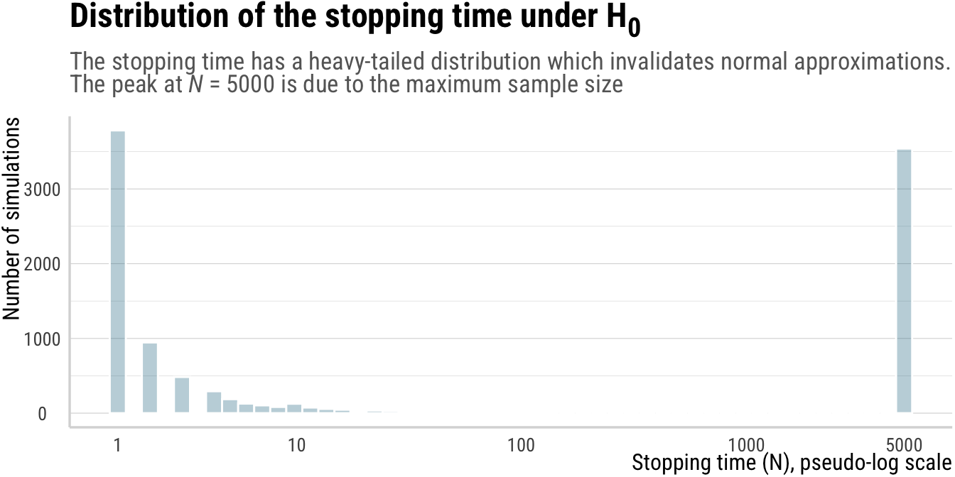

Now compare the likelihoods for the two experiments. The likelihoods are proportional, and thus the same inference about \(\mu\) should be drawn from both experiments, even though the sampling distributions differ.

mu_grid <- tibble(mu = seq(-0.5, 0.8, length.out = 500))

lik_df <- mu_grid %>%
    mutate(
        lik_fixed = exp(-n * (c - mu)^2 / (2 * sigma^2)),
        lik_stop = exp(-mean(stop_df$N) * (c - mu)^2 / (2 * sigma^2))
    ) %>%
    # normalize the likelihoods to max 1 to get rid of constants which don't matter for the likelihood principle
    mutate(
        lik_fixed = lik_fixed / max(lik_fixed),
        lik_stop = lik_stop / max(lik_stop)
    ) %>%
    pivot_longer(
        cols = starts_with("lik"),
        names_to = "design",
        values_to = "likelihood"
    ) %>%
    mutate(
        design = recode(
            design,
            lik_fixed = "Fixed sample size",
            lik_stop = "Optional stopping"
        )
    )

p_4 <- ggplot(lik_df, aes(x = mu, y = likelihood, lty = design)) +
    geom_vline(xintercept = c, color = colors[2]) +
    geom_line(linewidth = 1, color = colors[1]) +
    labs(
        title = "Observed data induce the same Gaussian likelihood",
        subtitle = "Once the observed mean is fixed (indicated by red line), the likelihood is proportional",
        lty = "Design",
        x = "Sample mean",
        y = "Relative likelihood"
    )
p_4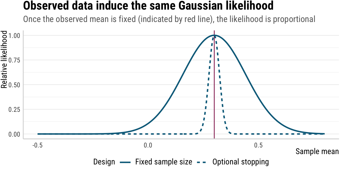

A brief aside regarding the narrower likelihood for the stopping scenario: Under known variance, the stopping rule is irrelevant for inference about \(\mu\). However, under unknown variance, the stopping rule is informative and sharpens inference. Once you enlarge the model from \(\mu\) to \((\mu,\sigma^2)\) using a distributional model approach (see Kneib et al. 2023; see also Thalmann in progress; Thalmann and Matticchio submitted for examples from experimental semantics), you have changed the inferential question and the stopping rule genuinely adds information about \(\sigma^2\). Here, however, we keep \(\sigma^2\) known to isolate the effect of the stopping rule on inference about \(\mu\) alone. Put more simply: when variance is estimated rather than fixed, the stopping time itself becomes informative, so the likelihoods are no longer proportional.

Why the \(p\)-values differ

Above, we saw that the likelihoods for the two experiments are proportional, and thus inference about \(\mu\) should be the same under both experiments. Now it is time to see why \(p\)-values differ between the two experiments, and thus why frequentist inferences based on \(p\)-values violate the likelihood principle. Suppose we test the null hypothesis \(H_0\) that \(\mu = 0\) using standard Null Hypothesis Significance Testing (NHST) procedures using \(p\)-values.

In Experiment A, where the sample size is fixed at \(n\), the sampling distribution of the sample mean under \(H_0\) is Gaussian:

\[ \bar X_n \sim \mathcal{N}\left(0, \frac{\sigma^2}{n}\right) \quad \text{under } H_0. \]

The \(p\)-value is

\[ p_A = P_0(|\bar X_n| \ge |c|) = 2\Phi\left(-\frac{|c|\sqrt n}{\sigma}\right). \]

In Experiment B, on the other hand, the sample size \(N\) is random and the event \(\bar X_N = c\) encodes a threshold: the sample mean stayed below \(c\) until time \(N\), then crossed it.

Therefore the null distribution of \(\bar X_N\) is not Gaussian, which makes it so that the resulting \(p\)-value differs from \(p_A\), typically being smaller. Thus, \(p_A \neq p_B\) despite identical likelihoods.

Let’s see why this is the case. Formally, a classical \(p\)-value is defined as

\[ p = \Pr_{H_0}(T \ge T_{\text{obs}}) \]

where \(T\) is a some statistic, \(T_{\text{obs}}\) is the observed value of that statistic, and the probability is taken under the null hypothesis \(H_0\). It is thus the probability of observing a test statistic as extreme or more extreme than the one observed, under the null hypothesis. The term more extreme is defined over all possible outcomes of the experiment. Thus, two experiments with proportional likelihoods yield different \(p\)-values because the inference depends on unobserved sample paths, and this directly contradicts the likelihood principle.

A little more technically, the crucial assumption is that the distribution of \(T\) under \(H_0\) is fully specified before observing the data and does not depend on how the data were collected, except through the final value of \(T\). But when the distribution of \(T\) depends on the data in some way, i.e., because we decide when to stop collecting data based on some summary statistic, then \(T\) is no longer fully specified under \(H_0\) before seeing the data.

Optional stopping introduces data dependence at the design level, rather than just at the level of the analysis. The stopping rule creates a situation where the distribution of \(T\) under \(H_0\) is not fixed in advance, but rather depends on the observed data and the stopping rule itself. This means that the reference distribution for \(T\) under \(H_0\) is not the same as it would be under a fixed sample size design, and thus the \(p\)-value calculated using the fixed-sample reference distribution will be incorrect.

As a result, the distribution of \(T\) under \(H_0\) is now a mixture over sample sizes, which depends on the stopping rule. Two identical final values \(T_{\text{obs}}\) may have very different probabilities under \(H_0\), depending on whether the statistic crossed the boundary early, whether it fluctuated near the boundary many times, and on whether it barely crossed at the last possible moment.

pvals <- tibble(
    design = c("Fixed sample size", "Optional stopping"),
    p_value = c(
        mean(abs(fixed_df$xbar) >= abs(c)),
        mean(stop_df$xbar >= c)
    )
)

p_5 <- ggplot(pvals, aes(x = design, y = p_value)) +
    geom_col(fill = colors[1], alpha = .3) +
    geom_hline(yintercept = 0.05, color = colors[2], linetype = "dashed") +
    labs(
        title = "Same observed mean, different *p*-values",
        subtitle = "*p*-values depend on the full sampling plan. Under the incorrect fixed-n reference distribution,<br>it looks unusual because the reference distribution for *as extreme as* is different. Under the<br>correct reference distribution, the observation is not unusual, hence the large *p*-value.",
        y = "Empirical *p*-value under H<sub>0</sub>",
        x = NULL
    )
p_5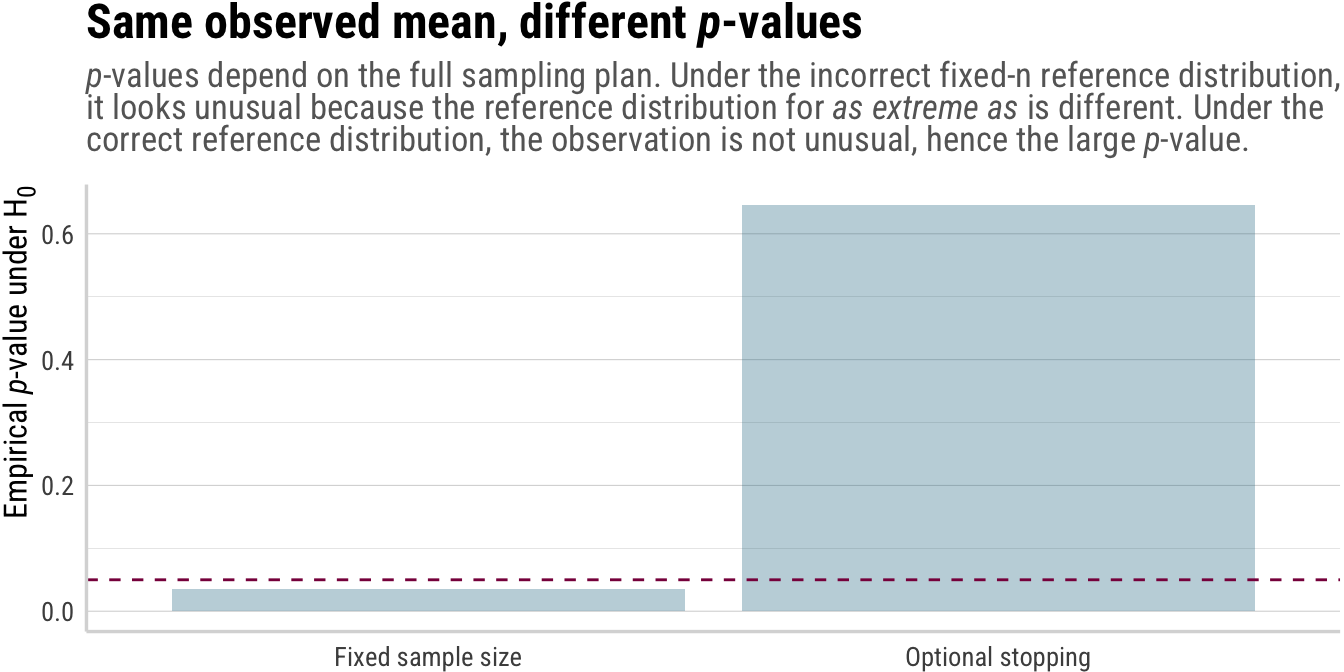

A summary: Tension between \(p\)-values and the likelihood principle

The likelihood principle states that inference about the validity of some hypothesis depends only on the likelihood, i.e., the data that we collected for the experiment. That is, no matter whether some data set \((X_1, \dots, X_n)\) was collected using one method or another, the amount of information for drawing inferences from the sample for the population (and accepting/rejecting hypotheses) is the same. Likelihood-based tests and Bayesian methods respect this equivalence.

As we saw above, however, \(p\)-values do not, because they rely on sampling distributions that change with the stopping rule. In effect, because \(p\)-values must consider how likely a result is under the assumption that the null hypothesis holds, they must take into account what outcomes would have been possible to begin with. And since stopping rules make completed datasets that do not fulfill the data-dependent condition impossible, stopping rules matter for the reference distribution and thus the \(p\)-value.

In other words, the invalidating assumption is that the test statistic’s null distribution is unaffected by data-dependent stopping. Optional stopping breaks this assumption, causing \(p\)-values to violate the likelihood principle. This tension is fundamental and cannot be resolved without abandoning either \(p\)-values or the likelihood principle.

References

Kneib, Thomas, Alexander Silbersdorff, and Benjamin Säfken. 2023. Rage against the mean: A review of distributional regression approaches. Econometrics and Statistics 26. Elsevier BV: 99–123. https://doi.org/10.1016/j.ecosta.2021.07.006.

Thalmann, Maik. in progress. Not so squeamish, Your majesty: The presuppositions of singular definites between existence and uniqueness.

Thalmann, Maik, and Andrea Matticchio. submitted. Kleene’ing up your attitude: Against universal presupposition projection.

Wagenmakers, Eric-Jan. 2007. A practical solution to the pervasive problems of \(p\) values. Psychonomic Bulletin & Review 14. Springer Science; Business Media LLC: 779–804. https://doi.org/10.3758/bf03194105.

Wagenmakers, Eric-Jan, Quentin Frederik Gronau, and Joachim Vandekerckhove. 2019. Five bayesian intuitions for the Stopping Rule Principle. Center for Open Science. https://doi.org/10.31234/osf.io/5ntkd.

Footnotes

1. In the data and throughout the blog post, I will differentiate between the two kinds of sample sizes by using \(n\) for the fixed sample size and \(N\) for the random sample size under optional stopping.